The data
The dataset comes from OP3, an open podcast analytics service that publishes anonymized download counts. We use a 2,414 × 142 matrix. Rows are podcast shows. Columns are listening apps and devices. Each cell is the number of times that show was downloaded through that app over the observed window.
90% of (show, app) pairs are unobserved, meaning most shows aren't listened to on most apps. That sparsity is what makes recommendation interesting. The model has to predict the empty cells from the patterns it sees in the filled ones.
Download distributions are heavy-tailed (a few huge shows, a long tail of small ones), so counts are log-transformed before fitting. All accuracy numbers on this page are in log space.
Hidden block structure
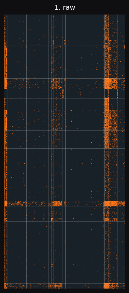
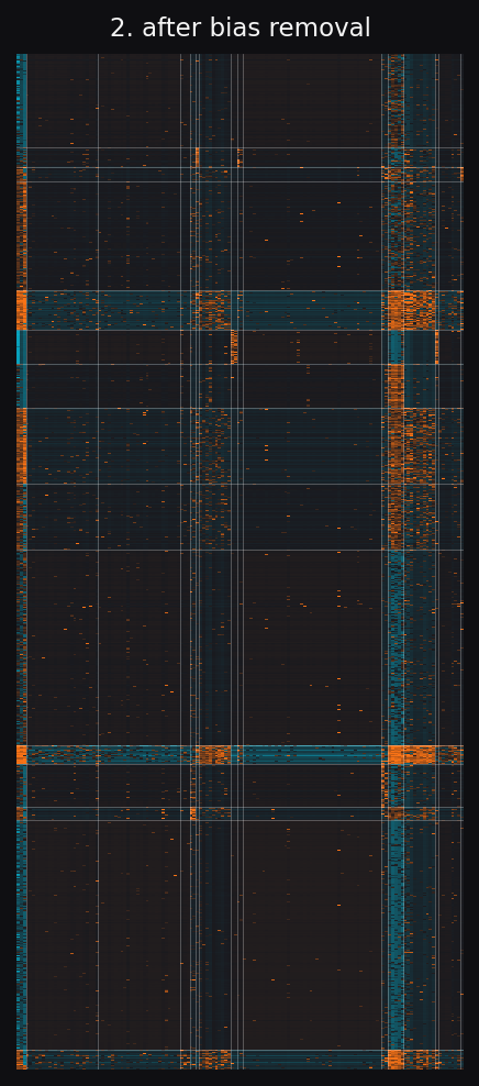
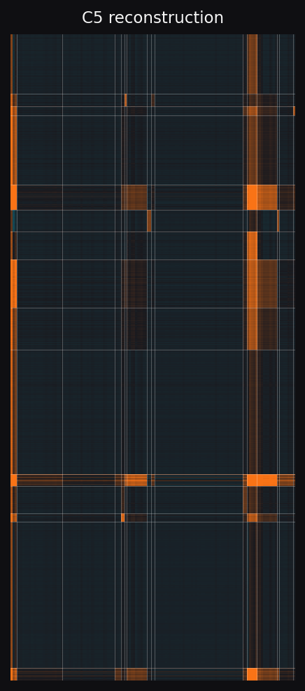
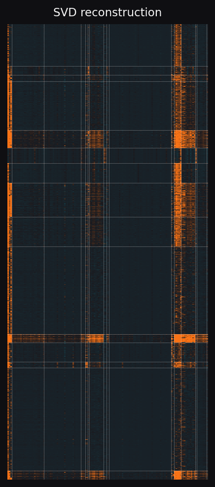
The raw matrix doesn't look structured because two effects dominate it. A few shows are huge. A few apps are huge. Subtract those biases out and a block pattern appears. Groups of shows that share an audience pattern with groups of apps. C5 fits this directly. SVD smooths over it.
Left to right: raw matrix, residual after subtracting show and app bias, C5 reconstruction, SVD reconstruction. Same row and column ordering throughout, recovered by C5.
Key Result
The block shape in panel 2 is the structure C5 fits. SVD predicts a continuous low-rank surface, so it smears block edges across many ranks. The accuracy gap later in the page comes from this shape mismatch.
Sixteen ways to listen
On the app side, C5 grouped the 142 apps into 16 clusters. Apps in the same cluster get downloaded in similar proportions across shows. The distribution is heavily skewed. The top two clusters cover 89% of all downloads. The long tail of 14 specialty and regional clusters covers the remaining 11%.
77.3%
3 apps
Apple Podcasts, Spotify, CastBox
11.8%
5 apps
Overcast, Pocket Casts, Podcast Addict, AntennaPod, Unknown Apple App
6.4%
10 apps
Amazon Music, Alexa devices, iHeartRadio, Audible, +6
0.9%
26 apps
NPR, Twitter, Xiao Yu Zhou, Anghami, +22
0.9%
10 apps
Podcast Guru, YouTube Music, Snipd, gPodder, +6
0.7%
23 apps
Podverse, MixerBox, radio.de, Roku, +19
0.3%
2 apps
iVoox, Deezer
0.3%
2 apps
Facebook, Google Podcasts
Top 8 clusters by download share. The remaining 8 clusters cover specialty, regional, and legacy apps.
A split within the mainstream
The most interesting finding sits inside the top two clusters above. Both groups are dominated by mainstream listening platforms. This isn't a "popular apps vs. obscure apps" split. The algorithm separated them because their audiences listen differently.
77.3%
Apple Podcasts, Spotify, CastBox
Platform-default listening. Audiences who consume podcasts through the app that came with their phone or their music service. Broadly matches the global category mix. This cluster is the average.
11.8%
Overcast, Pocket Casts, Podcast Addict, AntennaPod, Unknown Apple
Audiences who chose a dedicated podcast app. Smaller in share but consistent in pattern. Over-represented in tech and entrepreneurship. Under-represented in true crime and education.
Key Result
Two clusters cover 89% of all downloads. Co-clustering found a real audience difference inside platforms that look similar from the outside. That's the kind of finding single-axis methods would miss.
What each audience listens to
The heatmap below shows how each column cluster's listening pattern deviates from the global category mix. Values are lift, defined as the cluster's share of a category divided by the global share of the same category.
How to read lift. 1.0 means the cluster listens to that category at the same rate as the dataset average. Above 1.0 means over-represented. Below 1.0 means under-represented. The Apple+Spotify row sits close to 1.0 across most categories because that cluster contains 77% of all downloads, so the global average largely is it.
About the row labels. "Apple Podcasts + Spotify" is the name of a cluster, not two individual apps. The label uses the cluster's top two apps by download volume so you can recognize it. Each cluster contains multiple apps. See the ecosystem cards above for full membership.
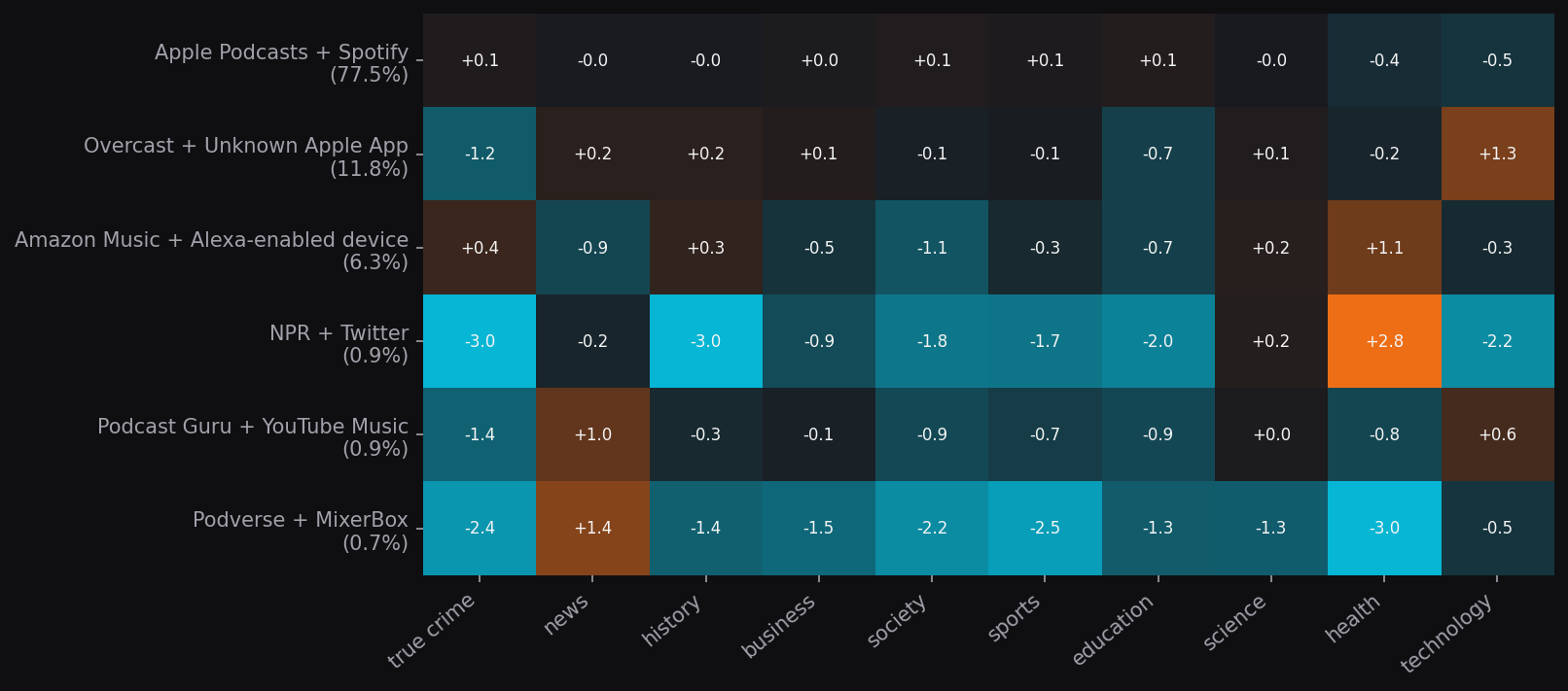
The strongest deviations sit in the smaller clusters.
- Dedicated podcast apps over-index ~4× on tech and entrepreneurship, ~3× on news. Under-index on true crime.
- Smart-speaker listeners (Amazon Music, Alexa devices, iHeartRadio) over-index on health and society.
- Walled-garden platforms (Apple+Spotify cluster) track close to 1.0 on every category. They are the global average.
Key Result
The 89% mainstream split looks uniform on the surface but breaks apart on category preference. Audience-shape differences this size are what single-axis methods would miss.
Audience habit, not topic
What organizes the row clusters? What makes two shows end up in the same group? We compared cohort's 15 row clusters against four candidate organizing axes using ARI (Adjusted Rand Index, the standard agreement metric between two clusterings, where 0 is random and 1 is perfect match).
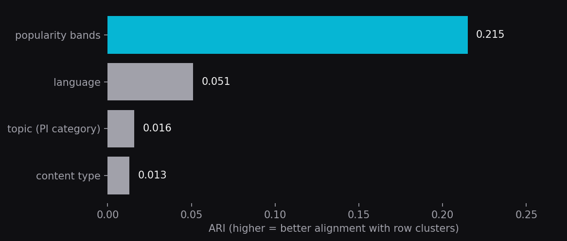
- Topic alignment (against Podcast Index categories like comedy, news, true crime): 0.016. Near random.
- Language: 0.051. Low signal.
- Content type (audio vs. video): 0.013. Low signal.
- Popularity bands: 0.215. The only candidate with real signal.
What "popularity bands" means here. We sort all 2,414 shows by total download volume (summed across all apps), then split them into deciles. Top 10%, next 10%, and so on. Each show's band is the decile it falls into. ARI of 0.215 against bands means the row clusters partition shows substantially along the "how big is this show's audience" axis.
Key Result
Cohort's row clusters group shows whose downloads come through a similar mix of apps at a similar scale. Two true-crime podcasts won't necessarily land in the same cluster. A true-crime podcast and a comedy podcast with similar download volume and similar app patterns probably will.
Prediction accuracy
Held-out MAE (lower is better predictions), averaged over five random seeds. C5 beats every baseline by a wide margin.
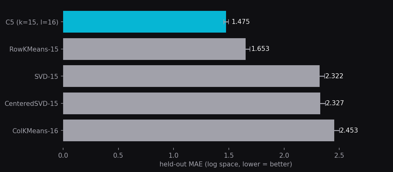
- C5 (k=15, l=16): 1.475 ± 0.021. The chosen model.
- RowKMeans-15: 1.653 ± 0.037. 12% worse than C5. Row-only clustering.
- SVD-15: 2.322 ± 0.046. 57% worse than C5. Truncated SVD baseline.
- CenteredSVD-15: 2.327 ± 0.047. 58% worse than C5. SVD with mean centering.
- ColKMeans-16: 2.453 ± 0.049. 66% worse than C5. Column-only clustering.
Key Result
The gap to SVD is 17 standard deviations across seeds. Signal, not noise. The gap to RowKMeans is the part of C5's advantage that comes specifically from co-clustering, meaning clustering shows and apps simultaneously rather than one axis at a time.
Why C5 wins
The block structure visible in the heatmap and the 36% accuracy gap over SVD come from the same fact. C5's predictor shape matches the data's shape.
C5: piecewise constant
Each (row cluster, column cluster) pair predicts one block-mean number. The whole prediction surface is a grid of flat blocks with sharp edges between them. That matches what the residual heatmap actually looks like.
SVD: smooth low-rank
Each cell is predicted from a continuous matrix product. The surface is smooth, good for gradients but bad for sharp edges. To express a block boundary, SVD has to combine many ranks. It can't fit all of them at low rank, so block edges get smeared.
Key Result
Shape match equals accuracy gap. The data is block-shaped. C5's predictor is too. SVD's isn't.
Picking k and l
How sensitive is the result to the choice of cluster count? We swept k ∈ {10, 15, 20, 25} for the row side and l ∈ {4, 8, 12, 16, 20} for the column side, measuring held-out MAE for each combination.
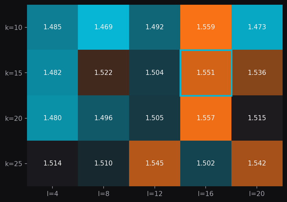
- Choice of cluster count: changes MAE by 6% across the swept grid.
- Choice of algorithm (C5 vs. SVD): changes MAE by 36%.
- Chosen settings (k=15, l=16, boxed in cyan): not a uniquely best point, but it surfaces the walled-garden split clearly with no measurable accuracy cost relative to neighbors.
Key Result
Algorithm choice matters about 6× more than cluster count. Once C5 is the algorithm, almost any reasonable (k, l) works.
How it scales
Two regimes, two winners.
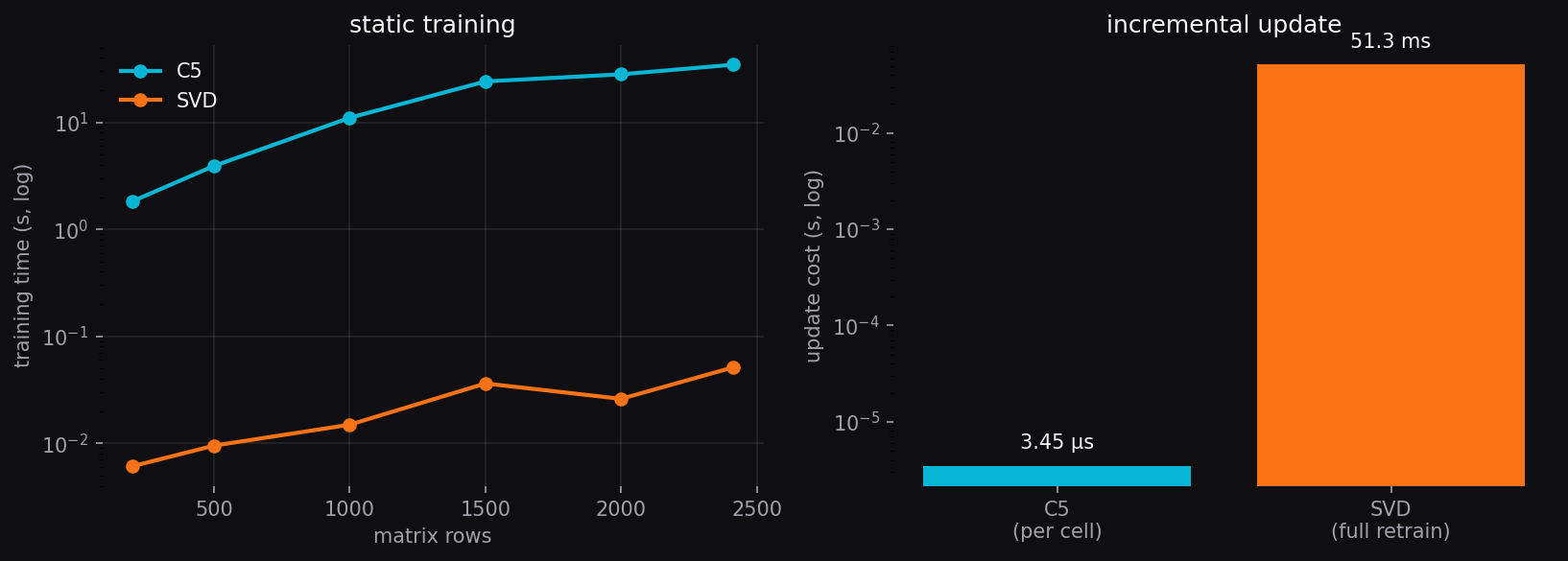
Static training: SVD wins
At our matrix size SVD fits in ~51 ms. C5 takes ~35 s. LAPACK's tuned linear-algebra primitives dominate at this scale. For one-shot training on a static dataset, SVD is dramatically cheaper.
Incremental updates: C5 wins
Adding one new download takes ~3.45 µs with C5's O(1) cell-update rule, versus a full SVD retrain at 51 ms. That's ~15,000× faster. The longer the dataset accumulates between full retrains, the more C5's incremental edge compounds.
Key Result
SVD wins one-shot. C5 wins streaming. For a recommender that has to incorporate fresh download data continuously, the streaming regime is the one that matters.
How it stays current
Recommendations have to stay fresh as new shows publish and new download data arrives. Cohort runs a two-tier refresh.
Weekly: incremental update
Pull the new week's OP3 download data. Existing shows update their audience profile in place via O(1) cell updates. Shows that are new to the dataset go into a transitional cluster (G&M's cold-start mechanism) and start appearing in recommendations immediately, before any retrain.
Monthly: full retrain
Rebuild all clusters from scratch. New arrivals settle into their final cluster homes. The slide deck has the pipeline diagram.
This is the load-bearing piece of running co-clustering in production. Without it, a fresh model would need a multi-hour retrain every time a new show landed. With it, new content gets a sensible audience profile on day one.
What didn't work
Four angles we tested that returned negative or weak results.
Topic-based grouping
Row clusters were not predicted by Podcast Index categories (true crime, comedy, news, etc.). ARI 0.016, indistinguishable from random. The clusters track app-distribution patterns and download scale, not subject matter. If you want a topic-similarity recommender, this isn't the model.
Show similarity from C5 output
Computing cosine similarity directly on C5's reconstructed rows collapses the space. The 2,414 shows compress into only ~240 distinct prediction patterns (k × l block means), so cosine sees most shows as near-identical. For show-to-show similarity, compare the raw log-download patterns instead.
Pearson on raw counts
The download distribution is heavy-tailed enough that any two big shows look correlated just by being big. Log-transforming before computing correlation fixes this. All accuracy numbers on this page assume the log transform.
Long-tail re-clustering
Re-running C5 on just the long-tail clusters didn't surface coherent sub-structure. The negative ARI against topic categories held up at finer resolution. The "audience habit, not topic" finding is robust to that re-cut.